
How to get click rates before we have clicks
Click-through rate (CTR) prediction is probably the most essential Data Science problem any online advertising company faces. The task is to estimate the probability that an impression with a certain set of features such as teaser text & image, weekday, placement, etc. will lead to a reader’s click. Obviously, this plays a critical role in the optimization of content delivery: The better and the earlier it is known what type of content works well with certain publishers, on which day/time and so on, the better campaigns can be personalized to the target audience. The basic concepts and a brief literature review of this dynamic field of research are presented in this article.
Modeling basics
CTR prediction is a supervised learning task, that means the problem is to learn a mapping from a set of features X (e. g, product category, publisher or weekday, …) of every impression to the CTR p, which is the probability that an impression with features X will lead to a click.
Since the CTR p is defined as the probability of a click to happen, it is a number that is always between 0 and 1 (or 0 and 100%). As an example of how such data should be modeled, imagine we live in a strange world where teaser CTRs strongly depend on the number of characters in the teaser title, with longer titles leading to higher click-through rates. We play out a series of teasers with different title lengths for a while and gather some clicks and (that’s life) some bounces. If we encode the clicks and bounces as 1 and 0, respectively, and draw them into a coordinate system with the title length on the x-axis, they may look like the orange dots in Figure 1.
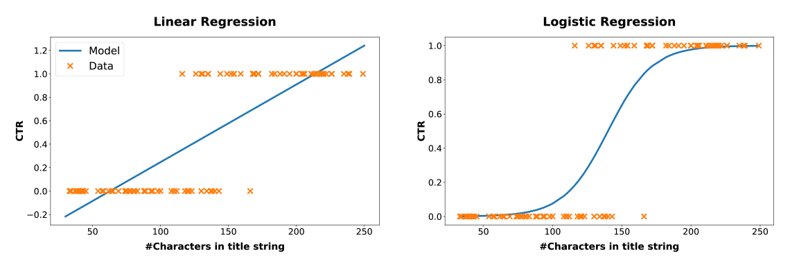
Figure 1: Linear and logistic regression with binary data. Linear regression leads to inconsistent predictions with click rates possibly smaller than 0 or larger than 1.
A simple and very tractable class of models is linear regression, where the target variable (CTR p) is modeled to be linearly dependent on the features, which in our example are the number of characters in the title string. Training a linear model typically consists of finding the line that minimizes the squared distance to the data points. Although linear regression can lead to pleasant results in many problems, it does not do the job in our case. It poorly matches the data and even worse, it is inconsistent: predictions of CTRs less than 0 or greater than 1 may occur, see the blue line in the left part of Figure 1.
In contrast, there is logistic regression (see the right part of Figure 1) which is the standard approach for data with target variables that model probabilities. We can see how much better logistic regression fits the data, with the CTR always between 0 and 1 as it necessarily must be. Instead of the squared distance to the data points, logistic regression maximizes the likelihood function of the corresponding Bernoulli process, ![]() , where p(Xn) is the predicted CTR for an impression with features Xn , typically modeled with a logistic sigmoid,
, where p(Xn) is the predicted CTR for an impression with features Xn , typically modeled with a logistic sigmoid, ![]() where the weight parameter w is learned from the training data. These equations might look cryptic if you don’t have a technical background, but the illustration of the comparison to linear regression in Figure 1 should be tangible for everyone.
where the weight parameter w is learned from the training data. These equations might look cryptic if you don’t have a technical background, but the illustration of the comparison to linear regression in Figure 1 should be tangible for everyone.
Of course, logistic regression can be used not only with one, but with any number of features X. Moreover, the linear model w · Xn in the exponent of the logistic sigmoid modeling the CTR p(Xn) can be replaced by any arbitrary more complex function, e. g., an artificial neural network. In a Deep Learning context, people usually talk about Binary Cross-Entropy Loss, referring to exactly the topic discussed above. In fact, the most popular modern CTR prediction models are Deep Learning models trained on binary cross-entropy.
Data and available features
Technically, one needs to distinguish between sparse and dense features. Dense features are numerical properties such as the number of characters in the title or the size of the image of a teaser. Sparse features are categorical labels, such as the weekday or publisher_id of an impression. They are called sparse because they are encoded with a sparse list of 0s and a single 1 labeling the category. For example, “weekday” would be a list with 7 entries where a “Thursday” is encoded as because it is the 4th day of the week. For several reasons, sparse features are cumbersome to work with. An obvious reason is that they cannot transfer similarities between similar categories. In the sparse weekday encoding, a Thursday is not more similar to a Wednesday than it is to a Sunday1. Moreover, every category of a feature leads to a new element in the feature vector, which is why the dimension of the feature vector X can quickly blow up to very large sizes.
Nonetheless, sparse features are ubiquitous in CTR prediction. We label advertisers with advertiser_ids, publishers with publisher_ids, publishers label their pages with channel_ids, placement_ids, and so on. Naively, even content may be sparsely encoded with title_ids, image_ids, etc. This typically leads to large, sparse feature vectors, a larger number of model parameters (beware of overfitting!), and the corresponding computational intricacies. Moreover, no information is transferred between similar samples like, e. g., two sparsely encoded teaser titles that only differ in a single word or a few characters.
A remedy for this problem, at least for text features like teaser title, body text, or even a category label for campaigns, is to use pre-trained text embedding systems like FastText, Universal Sentence Encoder, or BERT, which is currently revolutionizing natural language processing and probably worth another blog article. Essentially, these systems can transfer sparse features into dense ones, taking semantic similarities into account. However, many features like, e. g., advertiser_id or placement_id cannot be embedded by pre-trained models. It is therefore a major concern of today’s research on the topic, especially in the context of feature interaction, i. e., the interplay of title with image, content with weekday and so on.
Current research activities
Of course, Deep Learning found its way also into click-through rate prediction research. Deep Learning models can have millions of trainable parameters, which is the reason why they are so amazingly flexible. On the other hand, the more parameters, the more data and time is typically needed for model training. The research focus is therefore to create structured models, with the same expressivity but more compact model sizes. The central point is to model feature interactions without blowing up model complexity too much. For instance, finding out that a campaign on diapers may work particularly well on “eltern.de” would naively require the outer product between all campaigns and all placements. For example, with 1000 campaigns and 500 placements in the data, this means 500 · 1000 = 500.000 additional features for campaign-placement interaction alone. Model architectures to alleviate this issue are given by, e. g., Alibaba’s Deep Interest Networks, Google’s Wide & Deep (see Figure 2) or Microsoft’s DeepCross Networks.
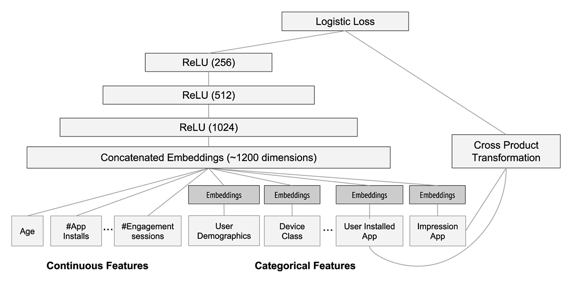
Figure 2: Architecture of Google’s Wide & Deep model for App recommendations. Taken from the original paper, https://dl.acm.org/doi/pdf/10.1145/2988450.2988454
Another important research direction is given by Bayesian/probabilistic models yielding probability distributions as predictions, a.k.a. “enabling your model to say ‘I don’t know’”. Having uncertainty measures on predictions is essential to drive content exploration: To learn most efficiently, we need to display impressions from time to time of which we just don’t know if they will work well or not. This is difficult to achieve with complex Deep Learning models, precisely because of their large number of parameters. As a result, this direction has been somewhat out of the limelight with the advent of Deep Learning. Work on this can be found in, e. g., Microsoft’s Web-Scale Bayesian CTR Prediction or the classic paper Simple and Scalable Response Prediction for Display Advertising developed at YahooLabs.
Conclusion
In this article, we learned that click-through rate prediction models are trained by maximizing the likelihood function, which is, loosely speaking, the probability of observing the clicks & views given the prediction model. We have seen that this objective can be combined with a large class of machine learning models, such as artificial neural networks. The data typically consist of dense features (e. g., number of characters in the title) and a large set of sparse features (e. g., advertiser_id, medium_id, etc.). Sparse features introduce some difficulties, especially in modeling feature interaction, which is currently the most vivid research direction.
Finally, a good CTR prediction model is the key component for optimizing campaigns across our publisher network: the more accurately we can predict the CTR, the more precise the targeting will be to the most susceptible audience.
1 Of course, one could find a dense encoding by labeling the weekdays, e. g., with numbers from 0 to 6, at the price of treating a Monday (0) maximally different from a Sunday (6).